Linear Regression Made Easy - How Does It Work And How to Use It in Python?

All you need to know about building Machine Learning models using the linear regression algorithm

Intro

Machine Learning is making huge leaps forward, with an increasing number of algorithms available so we can solve complex real-world problems.

This story is part of a deep dive series explaining the mechanics of Machine Learning algorithms. In addition to giving you an understanding of how ML algorithms work, it will also provide you Python examples so you can use them to build your own ML models.

What is covered in this story?

• What category of algorithms does linear regression belong to?

• What problems can be solved using linear regression?

• How does the linear regression algorithm work?

• How can I use linear regression to build a model in Python?

Linear regression algorithm

If you are only beginning your data science journey, then linear regression is the best place to start. It is a relatively simple algorithm that can be intuitively understood by everyone. I also provide graphs in this story that will help you to visualize it.

What category of algorithms does linear regression belong to?

The term "Machine Learning" is quite generic as it covers a huge number of algorithms. Hence, the first step is to find out which type of algorithms linear regression belongs to. Knowing that will give you a good idea of what problems you can use it for.

Side note, I have put Neural Networks in a category of their own due to their unique approach to Machine Learning. However, they can be used to solve a wide range of problems, including but not limited to classification and regression. The below chart is interactive so make sure to click👇 on different categories to enlarge and reveal more.

If you enjoy Data Science and Machine Learning, please subscribe to get an email whenever I publish a new story.

Linear regression is part of the supervised learning family, which means that the algorithm is trained using labeled data points. This is opposed to unsupervised techniques where algorithms use unlabeled data.

Supervised learning algorithms aim to model a relationship between one or multiple inputs (independent variables) and the output (dependent variable, a.k.a. target variable). For example, identifying the relationship between the size (sq.ft.) of the apartment and its market value.

Note, supervised learning is further split into classification and regression where:

• Classification is used to predict a class label. In other words, it is used for problems where the output (target variable) can be described by a finite set of values. For example, you can train a model to tell you whether an animal is a dog or a cat based on data inputs such as weight, height, tail length, etc. It is important to note that your model will only predict class labels that it has been trained to predict. I.e., if your model was trained to identify cats and dogs, then it will not be able to identify a mouse.

What problems can be solved using linear regression?

You can see how knowing your algorithm's category enables you to identify what problems you can use it for. In simple terms, any problem with the output being a numerical value can use linear regression.

In addition to the apartment value prediction mentioned above, here are several other examples:

• Predicting taxi fare based on distance traveled

• Predicting rainfall based on time of the year and location

• Predicting the homicide rate in the area based on income level and the prevalence of gun ownership

How does the linear regression algorithm work?

Linear regression models are often fitted using the least-squares approach. This requires finding the values of the parameters described in a linear equation of the 'best-fit line,' which is achieved by minimizing the sum of squared residuals.

While this may sound complicated, the logic behind it is quite simple. Instead of describing it with maths equations, let us look at the below chart. Black dots are the observations, the red line is the best-fit line, and the thin green lines are the residuals.

The linear regression algorithm's goal is to find a line (in this case, the red line) that has as many observations as close to the line as possible. This is what minimizing the sum of squared residuals is.

Since the above example is for a simple linear regression (only 1 input variable), the best-fit line would have the following equation y=ax+b, where y is the output (dependent) variable, x is the input (independent) variable, and a and b are the parameters known as slope and intercept.

Note, linear regression is not limited to using only 1 input variable. In fact, you can use as many input variables as you like. This is known as multiple linear regression, and I will give you an example of it in the Python section below.

How can I use linear regression to build a model in Python?

The two examples in this section are:

• simple linear regression (using 1 input variable)

• multiple linear regression (using 2 input variables). Note, I chose 2 input variables instead of, say, 5 because I wanted to draw a chart to help you visualize the solution. However, multiple linear regression can handle as many inputs as you like.

Also, both examples use the following:

• House price data from Kaggle

• Scikit-learn Python library to build linear regression models

• Plotly library for visualizations

Setup

First, let us import the required libraries.

import pandas as pd # for data manipulationimport numpy as np # for data manipulationfrom sklearn.linear_model import LinearRegression # for creating a modelimport plotly.graph_objects as go # for visualizationsimport plotly.express as px # for visualizations

Next, we download and ingest the data (source: https://www.kaggle.com/quantbruce/real-estate-price-prediction?select=Real+estate.csv)

# Read data into a Pandas DataFramedf = pd.read_csv('Real estate.csv', encoding='utf-8')# Print DataFramedf

Simple linear regression - Python example

For this model, we will take 'X3 distance to the nearest MRT station' as our input (independent) variable and 'Y house price of unit area' as our output (dependent, a.k.a. target) variable. Hence, the goal is to use the values of X3 to predict the value of Y.

First, let us create a scatter plot so we can see how these values are distributed.

# Create a scatter plotfig = px.scatter(df, x=df['X3 distance to the nearest MRT station'], y=df['Y house price of unit area'],                  opacity=0.8, color_discrete_sequence=['black'])# Change chart background colorfig.update_layout(dict(plot_bgcolor = 'white'))# Update axes linesfig.update_xaxes(showgrid=True, gridwidth=1, gridcolor='lightgrey',                  zeroline=True, zerolinewidth=1, zerolinecolor='lightgrey',                  showline=True, linewidth=1, linecolor='black')fig.update_yaxes(showgrid=True, gridwidth=1, gridcolor='lightgrey',                  zeroline=True, zerolinewidth=1, zerolinecolor='lightgrey',                  showline=True, linewidth=1, linecolor='black')# Set figure titlefig.update_layout(title_text="Scatter Plot")# Update marker sizefig.update_traces(marker=dict(size=3))fig.show()

As you can see, there is a noticeable relationship between the two variables. As the distance from the nearest MRT station increases, the price tends to decrease.

We will now run a simple linear regression model to find the best-fit line, which we can use to make predictions of price based on the distance to MRT.

# Select variables that we want to use in a model # Note, we need X to be a 2D array, hence reshapeX=df['X3 distance to the nearest MRT station'].values.reshape(-1,1)y=df['Y house price of unit area'].values# Fit linear regression modelmodel = LinearRegression()reg = model.fit(X, y)# Print the slope and intercept of the best-fit lineprint(reg.coef_)print(reg.intercept_)

The model has been fitted, giving us the slope of -0.00726205 and intercept of 45.85142705777498.

Now we can draw a best-fit line on the scatter plot.

# We will use below to draw a best-fit line on a chart# Create 20 evenly spaced points from smallest X to largest Xx_range = np.linspace(X.min(), X.max(), 20) # Predict y values for our set of X valuesy_range = model.predict(x_range.reshape(-1, 1))# Create a scatter plotfig = px.scatter(df, x=df['X3 distance to the nearest MRT station'], y=df['Y house price of unit area'],                  opacity=0.8, color_discrete_sequence=['black'])# Add a best-fit linefig.add_traces(go.Scatter(x=x_range, y=y_range, name='Regression Fit'))# Change chart background colorfig.update_layout(dict(plot_bgcolor = 'white'))# Update axes linesfig.update_xaxes(showgrid=True, gridwidth=1, gridcolor='lightgrey',                  zeroline=True, zerolinewidth=1, zerolinecolor='lightgrey',                  showline=True, linewidth=1, linecolor='black')fig.update_yaxes(showgrid=True, gridwidth=1, gridcolor='lightgrey',                  zeroline=True, zerolinewidth=1, zerolinecolor='lightgrey',                  showline=True, linewidth=1, linecolor='black')# Set figure titlefig.update_layout(title_text="Scatter Plot with Linear Regression Line")# Update marker sizefig.update_traces(marker=dict(size=3))fig.show()

As you can see, we now have a best-fit line for our model, which can predict a house price based on its distance from the MRT station. To get the prediction values, you can either use the predict() method or manually plug in a value of x into the line equation (y = -0.00726205*x + 45.85142705777498).

One additional observation from a chart above that you might have already spotted that highlights one of the limitations of linear regression. If we were to put an X value larger than 6,313, we would get a negative price, which is not realistic. A non-linear regression model could help us avoid this problem, but that is a topic for a future story.

Multiple linear regression - Python example

For this example, we will use the same data but add one more independent variable - 'X2 house age'. As before, let us first visualize the data. This time with a Plotly scatter 3D chart.

# Create a 3D scatter plotfig = px.scatter_3d(df, x=df['X3 distance to the nearest MRT station'], y=df['X2 house age'], z=df['Y house price of unit area'],                  opacity=0.8, color_discrete_sequence=['black'])# Set figure titlefig.update_layout(title_text="Scatter 3D Plot",                  scene = dict(xaxis=dict(backgroundcolor='white',                                          color='black',                                          gridcolor='lightgrey'),                               yaxis=dict(backgroundcolor='white',                                          color='black',                                          gridcolor='lightgrey'                                          ),                               zaxis=dict(backgroundcolor='white',                                          color='black',                                           gridcolor='lightgrey')))# Update marker sizefig.update_traces(marker=dict(size=3))fig.show()

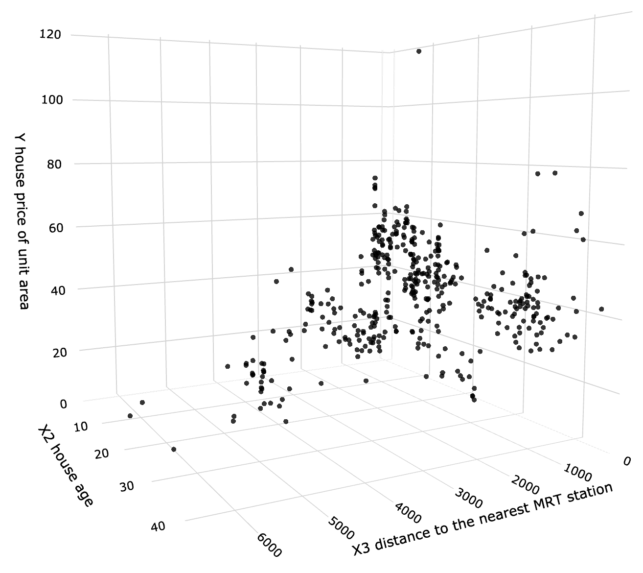
You can see from the above chart that the relationship also exists between the house age and price. This is great news as it will enable our model to give more accurate predictions. So, let's fit the model.

# Select variables that we want to use in a model # Note, X in this case is already a 2D array, hence no reshapeX=df[['X3 distance to the nearest MRT station','X2 house age']]y=df['Y house price of unit area'].values# Fit linear regression modelmodel = LinearRegression()reg = model.fit(X, y)# Print slope(s) and interceptprint(reg.coef_)print(reg.intercept_)

This time, since we have two independent variables, we get two slope parameters [-0.00720862 -0.23102658] and one intercept: 49.885585756906636. Again, you can use these to write a linear equation:

y = -0.00720862*[X3] -0.23102658*[X2] + 49.885585756906636.

The modeling here is done, but let us do a bit more work to plot the prediction plane onto our 3D graph. We will need to create a mesh with a range of input values and predict output values. This will give us the data for our plot.

# ------------------------ Prepare a number of points to use for prediction --------------------------# Increments between points in a meshgridmesh_size = 1# Identify min and max values for input variablesx_min, x_max = X['X3 distance to the nearest MRT station'].min(), X['X3 distance to the nearest MRT station'].max()y_min, y_max = X['X2 house age'].min(), X['X2 house age'].max()# Return evenly spaced values based on a range between min and maxxrange = np.arange(x_min, x_max, mesh_size)yrange = np.arange(y_min, y_max, mesh_size)# Create a meshgridxx, yy = np.meshgrid(xrange, yrange)# ------------------------------ Use the model to predict the output ---------------------------------# Run modelpred = model.predict(np.c_[xx.ravel(), yy.ravel()])pred = pred.reshape(xx.shape)# Note, .ravel() flattens the array to a 1D array,# then np.c_ takes elements from flattened xx and yy arrays and puts them together,# this creates the right shape required for model input# prediction array that is created by the model output is a 1D array,# we need to reshape it to be the same shape as xx or yy to be able to display it on a graph# ------------------------------------------- Plot --------------------------------------------------# Create a 3D scatter plot with predictionsfig = px.scatter_3d(df, x=df['X3 distance to the nearest MRT station'], y=df['X2 house age'], z=df['Y house price of unit area'],                  opacity=0.8, color_discrete_sequence=['black'])# Set figure title and colorsfig.update_layout(title_text="Scatter 3D Plot with Prediction Surface",                  scene = dict(xaxis=dict(backgroundcolor='white',                                          color='black',                                          gridcolor='lightgrey'),                               yaxis=dict(backgroundcolor='white',                                          color='black',                                          gridcolor='lightgrey'                                          ),                               zaxis=dict(backgroundcolor='white',                                          color='black',                                           gridcolor='lightgrey')))# Update marker sizefig.update_traces(marker=dict(size=3))# Add prediction planefig.add_traces(go.Surface(x=xrange, y=yrange, z=pred, name='pred_surface'))fig.show()

In the previous example, having one input variable gave us a 1D straight line - our prediction (regression) line.

Meanwhile, two input variables give us a 2D flat surface - a prediction plane. You can go up in dimensions by adding many more input variables to your model, which will work just fine, but you will not be able to draw a graph to visualize it.

To summarize, our final model is an improved one as it uses a combination of two variables to predict the house price. Try to practice by adding more input variables to see how good you can get your model.

Final Remarks

I hope you now have a clear understanding of how linear regression works, and you are keen to build your own prediction models.

I will continue the series with more stories about other Machine learning algorithms. If you have any suggestions on how I can make it better, feel free to reach out.

Cheers! 👏 Saul Dobilas

Related articles you may like:

MARS: Multivariate Adaptive Regression Splines - How to Improve on Linear Regression?

LOWESS Regression in Python: How to Discover Clear Patterns in Your Data?

Support Vector Regression (SVR) - One of the Most Flexible Yet Robust Prediction Algorithms