Greener green and bluer blue: Ocean poleward greening over the past two decades

We start by showing the well-known and distinctive spatial distribution of climatological Chl (Fig. 1, A and B). The elevated Chl (mean of 0.38 mg m⁻³) in the subpolar regions (40° to 60°) stands in sharp contrast to the relatively low Chl (mean of 0.074 mg m⁻³) in the oligotrophic gyres of the mid-latitudes (10° to 30°). In the tropics (0° to 10°), characterized by strong upwelling that boosts phytoplankton growth, the mean Chl is again elevated (mean of 0.14 mg m⁻³). To explore latitudinal trends, we calculated the annual mean Chl of each 2° latitudinal band between 60°S and 80°N from 2003 to 2022 and then used the Sen’s slope estimator to determine trends (methods). We found that Chl has significantly decreased at an average rate of 0.55% year⁻¹ in the northern subtropical region (20°N to 40°N) (Fig. 1C). In contrast, Chl shows increasing trends in both northern and southern subpolar regions at a rate of 0.28% year⁻¹ and 0.44% year⁻¹, respectively. Moreover, consistent with previous studies (16, 17), we found that the Arctic Ocean (66°N to 80°N) has experienced a significant increase in Chl at a rate of 1.99% year⁻¹. Collectively these results indicate a broad pattern whereby Chl is decreasing in the low-Chl waters of the subtropical and tropical regions while increasing in the high-Chl waters at higher latitudes (>40°).

To assess the relative contribution of these latitudinal bands to the total Chl in each hemisphere, we used a Lorenz curve and the corresponding Gini index, which were originally developed for economic analysis (methods). We examined the Northern Hemisphere (NH) and Southern Hemisphere (SH) separately because of the well-known differences in the dynamics that govern the high latitudes in these hemispheres. Given the distinctive environmental conditions in the Arctic Ocean and previous work in this region, we hereafter focused on analyzing the open ocean between 60°S and 60°N [see (16) for Arctic-specific trends]. As seen by the Lorenz curve, in which the 30 latitudinal bands are ranked in ascending order according to their contribution to the cumulative chlorophyll in each hemisphere, the subpolar latitudes (40°N to 60°N) place in the top 10 latitudinal bands in the NH (Fig. 2A), contributing 55.6% to the total. In contrast, the latitudinal bands between 20°N and 30°N fall in the 20th percentile, contributing only 8.1%. In the SH, the latitudinal bands with the largest contribution (28.3%) to the cumulative total are between 40°S and 50°S. They are followed by latitudes between 30°S and 40°S (18.8%), between 50°S and 60°S (18.2%), and 0° and 10°S (15.9%) (Fig. 2C). As seen here, the NH has a greater latitudinal disparity than the SH, mainly because Chl in the NH subpolar region exceeds that in the comparable SH region. This difference is likely mainly attributable to the known iron deficiency that limits phytoplankton biomass (18) in the high nutrient–low chlorophyll Southern Ocean.

From the Lorenz curve, we next calculated trends in the Gini index of area-integrated Chl over each latitudinal band from 2003 to 2022 for each hemisphere (methods; similar trends are observed with latitudinal averaged Chl, see fig. S1). We find a growing latitudinal disparity in Chl in the NH, as measured by a significant increase of 0.20% year⁻¹ in the Gini index. The significant increase of the Gini index tends to occur in the winter and autumn seasons (fig. S2), indicating a seasonal difference in the latitudinal disparity of Chl. In the SH, the increase is not statistically significant (despite an increase in Chl concentrations in the SH subpolar latitudes). One reason for this difference is that Chl has decreased significantly in the northern subtropical regions, where the relatively low Chl has become lower over the same period, whereas no such trends are detected in the SH. We note that our latitudinal binning masks a myriad of variability in Chl trends at regional and biome scales, with spatial heterogeneity in the magnitude and sign of linear trends, particularly in the southern subtropical regions. Although a local analysis is beyond the scope of our study, contrasting trends at the local level likely explain the absence of trends in certain latitudinal bands (e.g., SH subtropics). For further context, a comparison with recent literature on global ocean color trends that focuses on region is provided in the supplementary materials (table S1).

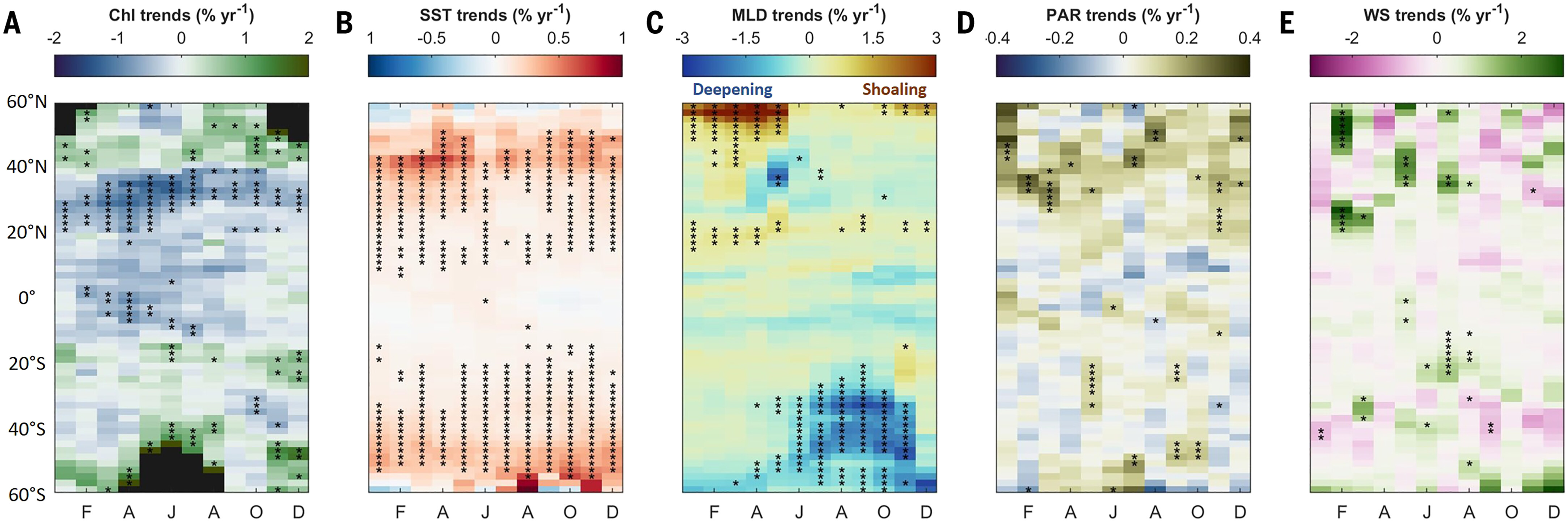
As a first approximation, we examined the trends of four environmental factors (Fig. 3) believed to critically influence Chl concentrations—sea surface temperature (SST), mixed layer depth (MLD), photosynthetically available radiation (PAR), and wind speed (WS)—and then determined the observed sensitivity of Chl to these factors. A few patterns stand out from the comparison of trends. In the northern subpolar regions (40°N to 60°N), where significant increases in Chl are primarily detected from October to February at a rate of 0.88 ± 0.41% year⁻¹ (Fig. 3A), we note concurrent increases in SST and PAR (Fig. 3, B and D) as well as a shoaling in the MLD (Fig. 3C). In the northern subtropical region (20°N to 40°N), where Chl shows a year-round decreasing trend at a rate of −0.75 ± 0.25% year⁻¹, with significant changes observed in 56.7% of the region (Fig. 3A), SST shows significant increases throughout the year in 79.2% of the grids (Fig. 3B). Finally, in the southern subpolar regions (40°S to 60°S), where Chl has increased significantly in the months of April to August at a rate of 1.24 ± 0.64% year⁻¹, a few concurrent SST trends are also observed (Fig. 3, A and B).

The observed sensitivity of Chl trends to trends in the four environmental variables suggests that SST is a dominant factor for Chl changes in the subpolar region of both hemispheres and in the subtropics of the NH (Fig. 4). The increase in Chl in the subpolar regions is likely associated with the observed increase in autumn and winter blooms (19, 20), consistent with projected increases in net primary productivity driven by sea ice retreat, shoaling of mixed layers, and a reduction in light limitation (16, 21, 22), all tightly linked to the surface warming observed here. In the NH subtropics, the decreasing Chl trend and concurrent increasing SST trend are supported by in situ observations at the Bermuda Atlantic Time-series site (BATS). A previous study (23) found that rising SST reduces phytoplankton productivity in the oligotrophic ocean, putatively through a reduction in nutrient supply, a result consistent with increased stratification observed in recent years (24). The Southern Hemisphere subtropics do not exhibit a clear sensitivity to any of the variables, likely because the Chl trends here are the weakest across all latitudes (Fig. 3A). Finally, the lack of significant trends in the tropics for all environmental variables (Fig. 3, B to E) precludes any attribution of the decreasing Chl trend observed there (Fig. 4).

As mentioned above, complex dynamics in the ocean environment complicate the attribution of Chl changes. While our analysis suggests that broadscale SST changes are likely driving latitudinal Chl changes, our results are inconclusive for the three other variables studied here. Regional studies provide additional insights to this global analysis. For example, wind speed emerges as a significant factor in annual Chl variation across both tropical regions and eastern boundary currents (25, 26). In the tropical Indian Ocean, reduced wind speeds have been correlated with increased stratification, which suppresses nutrient upwelling, thus contributing to declining Chl. Conversely, in the California Current System, elevated wind speeds have been found to facilitate upwelling, thus enhancing phytoplankton biomass and fostering a “greening” effect. Modeling studies that incorporate these variables, and others such as turbulent mixing and aerosol deposition (7, 8), are needed to further elucidate the mechanisms driving the latitudinal Chl trends observed here.

It remains to be established whether the significant trends over the 20-year record reported here stem from natural variability over the satellite era or rather are driven by a changing climate. Previous studies suggest that satellite time series would need to be ~30 to 40 years in length to distinguish climate-driven Chl trends from internal variability (12, 27, 28). Because variations in Chl reflect both biomass and physiology (6), we cannot attribute the Chl trend to changes in phytoplankton biomass. However, our observations of poleward greening and increasing latitudinal disparity align with 21st-century projections of a sustained decrease in net primary productivity in the low- and mid-latitudes that is coupled with an increase in high-latitude areas (29, 30). Through trophic amplification, the decline in phytoplankton biomass associated with climate warming will have a more pronounced impact on biomass at higher trophic levels (31–33), with a projected decline in fish production and fisheries in the tropics and an increase in the high latitudes (34–36). More than 50% of the global fish catch comes from tropical and subtropical regions, with significant contributions from coastal fisheries (37). Although our study focuses on open ocean waters, any persistent changes in these areas could profoundly affect low- and middle-income nations, such as Pacific Island nations, that rely on fisheries for sustenance and economic development (38, 39). Future investigations should focus on these regions to provide a more comprehensive understanding. In particular, it will be important to investigate how climate change, and climate mitigation through iron fertilization (40), could synergistically affect air-sea CO₂ fluxes and exacerbate fisheries inequity.

We thank K. Arrigo and G. Van Djiken for sharing the Arctic dataset on chlorophyll concentration. H.Z. thanks X. Kang for sharing insights about statistical methods.