ANOVA Test, with Python
The Complete Beginner's Guide to perform ANOVA Test (with code!)

In previous articles, I have discussed how to perform one-sample hypothesis tests and two-sample hypothesis test. So, what if we would like to compare several population means? In this article, I will introduce an analysis of variance (ANOVA) which involves comparing multiple unknown μ's.
One-Way ANOVA
It is a test where a particular factor has more than 2 groups or levels of interest. For example, let μ be the true mean annual salary of graduates
Single-factor of interest = Study subjects
Assume we have 6 categories of study subjects, Factor levels = athematics and Statistics, Economics and Finance, Environmental Sciences, Political Science, Social Sciences and Biology.
Hence, there are 6 levels or groups of this single factor in affecting the mean of the annual salary of graduates.
The basic idea behind a one-way ANOVA is to take independent random samples from each group, then compute the sample means for each group. After that compare the variation of sample means among the groups to the variation within the groups. Finally, make a decision based on a test statistic, whether the means of the groups are all equal or not.
Sum of Squares (SS)
Inside the One-Way ANOVA Table: The total amount of variability comes from two possible sources, namely:
Difference among the groups, called treatment (TR)
Difference within the groups, called error (E)
The sum of the squares due to treatment (SSTR) and the sum of squares due to error (SSE) are listed in the one-way ANOVA table. The sum of SSTR and SSE is equal to the total sum of squares (SSTO).

Just like for SS, d.f. (SSTO) = d.f. (SSTR) + d.f. (SSE)
Mean Squares (MS)
A mean square is the sum of squares divided by its d.f. These mean squares are all variances and will be used in the hypothesis test of the equality of all the group population means.
Assumptions for the one-way ANOVA hypothesis test
Sample data are randomly selected from populations and randomly assigned to each of the treatment groups. Each observation is thus independent of any other observation - randomness and independence.
Normality. Values in each sampled groups are assumed to be drawn from normally distributed populations. We can use normal probability plot or Q-Q plot to check normality.
Homogeneity of variance. All the c group variances are equal, that is σ₁² = σ₂² = σ₃² = ... = σ𝒸². As a rule of thumb, if the ratio of the largest to the smallest sample standard deviation is less than 2, we consider the equal standard deviations assumption as fulfilled.
The simple outline of the one-way ANOVA test:
F test for differences in more than two means H₀: μ₁= μ₂ = μ₃ = ... = μ𝒸 H₁: Not all μᵢ's are equal, where i = 1, 2, 3, ..., c. Level of significance = α

Finally, the one-way ANOVA table is as shown below:

Given a students.csv dataset consists of 8239 rows, each of them representing a particular student, and 16 columns (stud.id, name, gender, age, height, weight, religion, nc.score, semester, major, minor, score1, score2, online.tutorial, graduated, salary), each of them corresponding to a feature related to that particular student. Is there evidence of a significant difference in average annual salary for graduates of different study subjects at 5% significance level? There are 6 different study subjects.
Data Exploration and Preparation
From the dataset given, we first need to filter out the students who are graduated and do a random sampling process. In our case, we will randomly sample 500 students from the dataset using random.sample a function in Python. After that, we will our dataset to the two variables of interest, the categorical variable major and the numeric variable salary.

Normality Assumption Check
Before we perform the hypothesis test, we check if the assumptions for the one-way ANOVA hypothesis test are fulfilled. The samples are random and independent samples. Now, we check the normality assumption by plotting a normal probability plot (Q-Q plots) for each grouped variable.

The Q-Q plot shows a largely straight-line pattern if it is from a normal distribution. From the above figure, we may assume that the data for each group falls roughly on a straight line.
Homogeneity of variance Assumption Check

The ratio of the largest to the smallest sample standard deviation is 1.67. That is less than the threshold of 2. Thus, we conclude that the assumptions are fulfilled.
Hypothesis Testing
According to five steps process of hypothesis testing: H₀: μ₁= μ₂ = μ₃ = ... = μ₆ H₁: Not all salary means are equal α = 0.05 According to F test statistics:
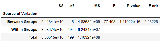

Conclusion: We have enough evidence that not all average salaries are the same for graduates of different study subjects, at 5% significance level.
Recommended Reading
Two-Way ANOVA Test, with Python
References
[1] "One-way ANOVA • SOGA • Department of Earth Sciences." [Online]. Available: https://www.geo.fu-berlin.de/en/v/soga/Basics-of-statistics/ANOVA/One-way-ANOVA/index.html
[2] "One-way ANOVA Hypothesis Test • SOGA • Department of Earth Sciences." [Online]. Available: https://www.geo.fu-berlin.de/en/v/soga/Basics-of-statistics/ANOVA/One-way-ANOVA-Hypothesis-Test/index.html